I recently presented a session about Google BigQuery at the Google Cloud Summit in Amsterdam. While preparing for the session I was reminded how easy it is to get started, at no cost and without a credit card, to explore your own data. In my presentation I showed a short demo working with a dataset I uploaded, and then combining it with a public dataset. This blog allows you to execute the demo yourself, for free!

In this 30 minute tutorial you will get experience with:

• Accessing Google Cloud and the free BigQuery sandbox
• Loading your own data from Cloud Shell
• Querying and visualizing your own data
• Using the geospatial capabilities of BigQuery to explore public weather data
• Combining your own and public weather data to make new visualizations

Are you ready? Let’s go!

[1] Login to Google Cloud

First thing is to get connected to Google Cloud. Use your existing Google (Gmail) account, or create a new one just to try this stuff out. Remember, you will not be charged anything, nor have to provide payment details to use the BigQuery Sandbox which gives you monthly up to 1 TiB of querying and 10 GiB of space for tables with a 60 day retention.

1. Load the BigQuery UI
2. If you want to create a new account do so now, otherwise login using your existing account.
3. Accept the Google Cloud Platform Terms of Service.
4. Click on the create project link and give it a name.
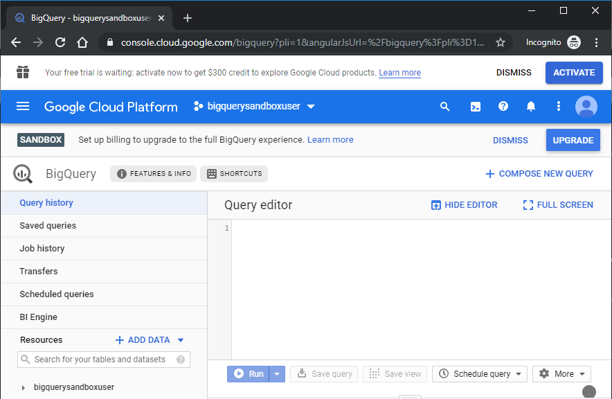
5. Done! You should see the BigQuery UI query editor ready to go!

[2] Run a query on a public dataset

There are tons of public datasets already loaded in BigQuery, so lets use one to make sure our environment is working. My personal favorite is a dataset of birth names in the USA since 1910. We can feed our curiousity and make sure things work at the same time :-)

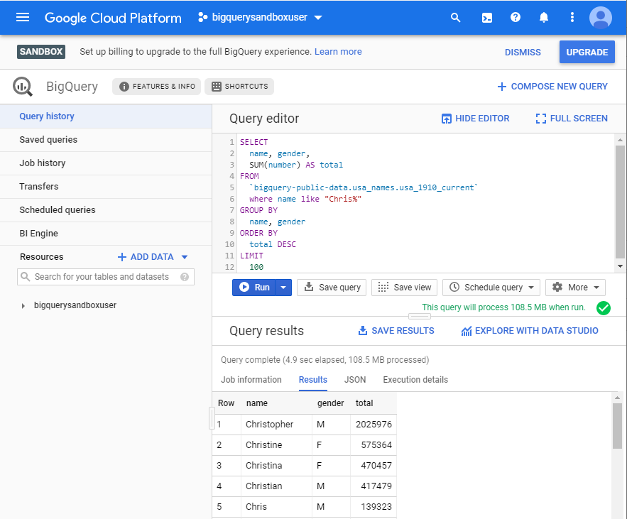
1. In the BigQuery UI enter the following query, replacing “Chris” with [part] of your own name to find names similar to your own, and hit Run:

   SELECT
   name, gender,
   SUM(number) AS total
   FROM
   `bigquery-public-data.usa_names.usa_1910_current`
   where name like "Chris%"
   GROUP BY
   name, gender
   ORDER BY
   total DESC
   LIMIT
   100
   

2. You should see results that look like something like this:

3. Celebrate that you name is more special than you thought, or cry if it’s less! Now it’s time to load some of your own data.

[3] Load some data.

Since I’m in The Netherlands I started scouting around on some open data sites and stubled upon parking transactions for the city of Arnhem. Hmm. I always wondered when parking garages are busiest so why not give it a try?

There are several ways to load data into BigQuery, with the most common one being from Cloud Storage. But, Cloud Storage requires at least a Google Cloud trial account [and payment details], and we didn’t do that. You can upload data from the BigQuery UI directly, but it’s limited to 10 MiB per file. Cloud Shell to the rescue! Cloud Shell is a free linux shell you can launch from the Cloud Console that will enable us to load bigger files.

1. Open up a Cloud Shell using the shell icon from the Google Console
2. In a new browser tab, open up the Arnhem parking data, and find the table that has Transactiedata - Parkeergarages

3. Download a file to Cloud Shell by right clicking on a parking data file, copy link, and paste into a wget command in your Cloud Shell. This is just one of the files, grab as many as you like:

   wget https://monitdata.s3.amazonaws.com/arnhem/offstreet/transactions/arnhem_opendata_offstreet_201908.csv
   

4. Create a BigQuery table for the parking data. Click on the project name and then the CREATE DATASET button

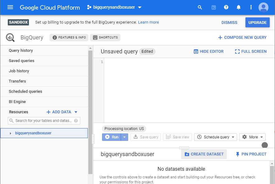
5. Set a dataset name of parking, do not modify the other options, and click Create dataset

6. From Cloud Shell we can create a table and load the data we downloaded a moment ago:

   bq load \
   --source_format=CSV \
   --skip_leading_rows=1 \
   --field_delimiter=';' \
   --replace=false \
   --autodetect \
   parking.data \
   ./arnhem_opendata_offstreet_201908.csv
   

7. A few seconds later your data is ready to be queried in BigQuery! Since we created the table from the CLI, refresh the browser tab for it to list the new table.

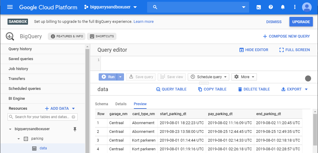
8. Expand the Resources tree to show the table, and click on the Schema, Details, and Preview tabs to get a better understanding of the data.

[4] Query your data

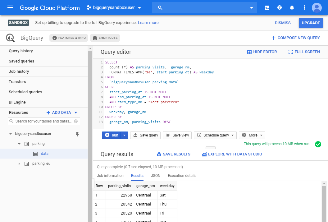
1. Clicking on the table, and then the preview tab, is a nice way to get a feel for the data format. I decided I’d like to see which day of the week is the busiest for each garage, for non subscription holders, and here’s the query I came up. Run it after changing the bigqueryusersandbox to your own project name:

   SELECT
   count (*) AS parking_visits,  garage_nm,
   FORMAT_TIMESTAMP('%a', start_parking_dt) AS weekday
   FROM
   `bigquerysandboxuser.parking.data`
   WHERE
   start_parking_dt IS NOT NULL
   AND end_parking_dt IS NOT NULL
   AND card_type_nm = "Kort parkeren"
   GROUP BY
   weekday, garage_nm
   ORDER BY
   garage_nm, parking_visits DESC
   

2. The results indicate Saturday, Thursday, and Friday are the busiest!

[5] Visualize your data

Scrolling through data in a table can be nice, but lets make it visual using Google Data Studio. Data Studio is a free data visualization tool from Google that has great integration with BigQuery! Let’s try to make a stacked bar chart with visits per day of the week per garage.

1. Click the Explore with Data Studio button and click through the prompts that appear.
2. The Data Studio interface Data tab is where you need to match up the graph view type and the source data from the table.
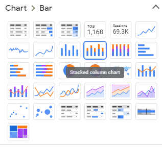
   1. First, click a stacked column chart
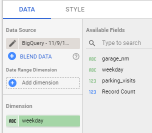
   2. Next, from the available fields list, drag and drop weekday to the Dimension field of your chart
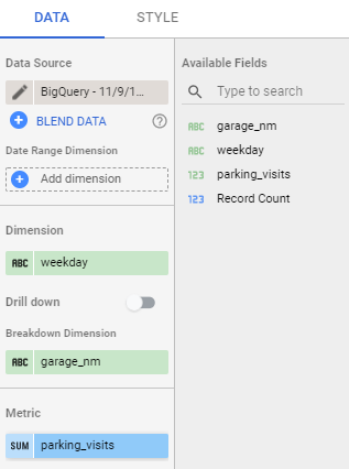
   3. Next, from the available fields list, drag and drop parking_visits to the Metric field of your chart
3. Check out the beautiful chart that visualizes the data. Looks like for the data I loaded the parking garage users are coming for fun and not work!
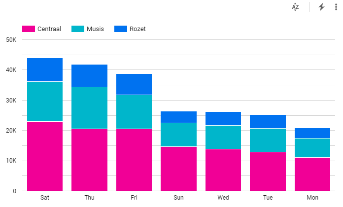
4. It’s possible to save this chart, and then share with other users, with a few more clicks. Easy does it!

[6] Combine your data with public data

Now that we have our own parking data loaded, lets try to combine it with Global Historical Climate Network (GHCN) weather data, one of the public datasets already loaded in BigQuery. This dataset includes historical weather data from over 80,000 stations in 180 countries.

1. First we need to find a weather station nearby Arnhem that is reporting. To do that, we need the latitude and longitude of the Centraal garage in Arnhem. An easy way is to search for it in Google Maps, and then right click on the garage and choose the “What’s here”. A small window appears with a photo of the location with the decimal latitude and longitude of it.

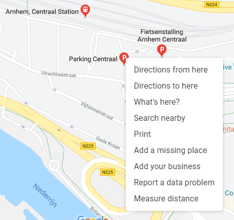
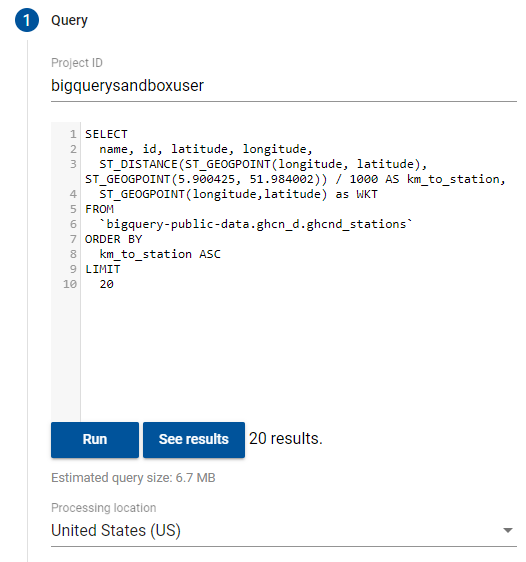
2. In BigQuery search for the closest 20 weather stations based on this latitude and longitude:

   SELECT
   name, id, latitude, longitude,
   ST_DISTANCE(ST_GEOGPOINT(longitude, latitude), ST_GEOGPOINT(5.900425, 51.984002)) / 1000 AS km_to_station,
   ST_GEOGPOINT(longitude,latitude) as WKT
   FROM
   `bigquery-public-data.ghcn_d.ghcnd_stations`
   ORDER BY
   km_to_station ASC
   LIMIT
   20
   

3. You can also see this visually using BigQuery Geo Viz. Visit this site, authorize it and pick your GCP project, paste in the same query, and set the Style -> circleRadius to 500:

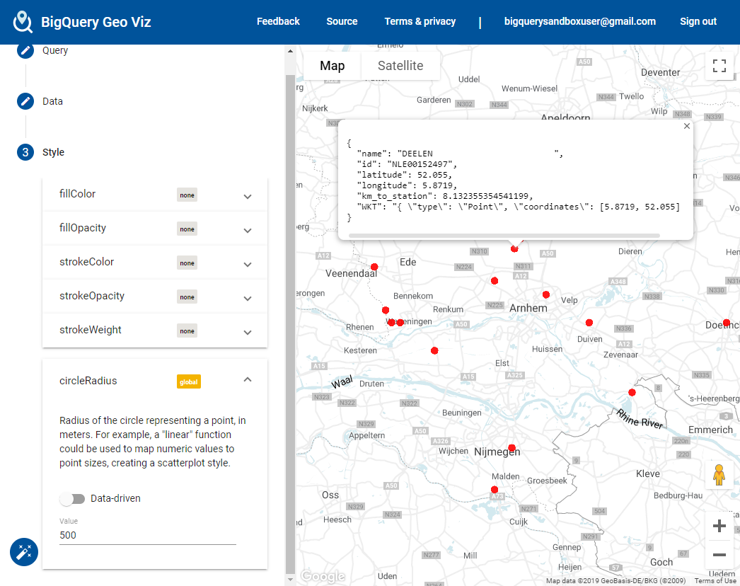
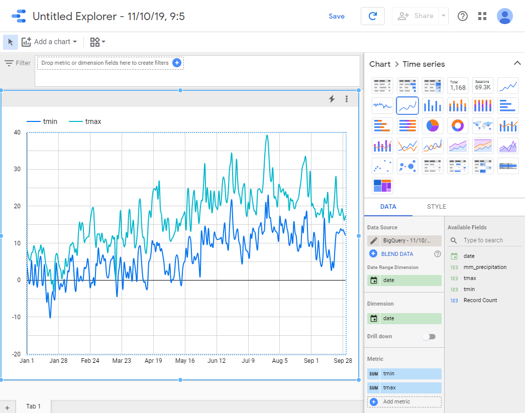
4. Not all stations have current weather, so take a quick look to make sure the station name you pick (in our case NLE00152497) is reporting:

   SELECT
   date,
   MAX(mm_precipitation) AS mm_precipitation,
   MAX(tmin) AS tmin,
   MAX(tmax) AS tmax
   FROM (
   SELECT
   w.date,
   IF (w.element = 'PRCP', w.value/10, NULL) AS mm_precipitation,
   IF (w.element = 'TMIN', w.value/10, NULL) AS tmin,
   IF (w.element = 'TMAX', w.value/10, NULL) AS tmax
   FROM
   `bigquery-public-data.ghcn_d.ghcnd_2019` AS w
   WHERE
   id = 'NLE00152497'
   AND qflag IS NULL )
   GROUP BY
   date
   ORDER BY
   date
   

   Note: Check here for a query that helps find reporting stations automatically

And, for fun, click the EXPLORE WITH DATA STUDIO button and setup the as below for a nice chart:

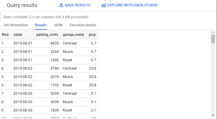
1. Now we can combine our parking data and the weather data:

   SELECT
   DATE(start_parking_dt) AS sdate,
   count (*) AS parking_visits,
   garage_nm AS garage_name,
   w.prcp
   FROM (
   SELECT
   date,
   value/10 AS prcp
   FROM
   `bigquery-public-data.ghcn_d.ghcnd_2019`
   WHERE
   id = 'NLE00152497'
   AND qflag IS NULL
   AND element = 'PRCP') AS w
   JOIN
   `bigquerysandboxuser.parking.data` AS p
   ON
   DATE(start_parking_dt) = w.date
   WHERE
   start_parking_dt IS NOT NULL
   AND end_parking_dt IS NOT NULL
   GROUP BY
   garage_name,
   sdate,
   prcp
   ORDER BY
   sdate
   

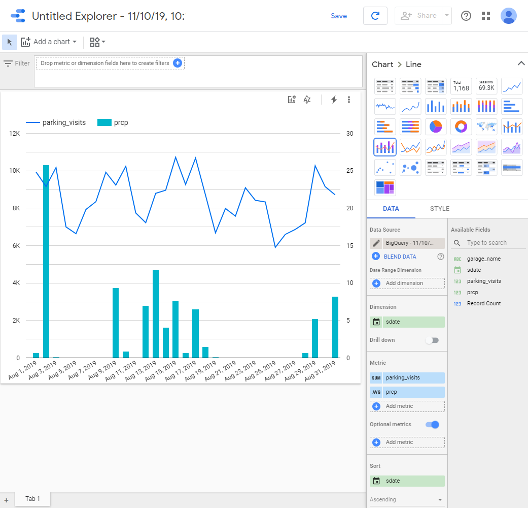
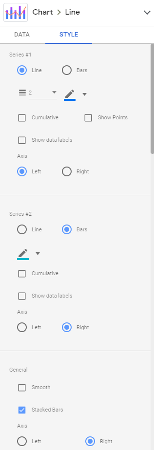
1. And finally, click the EXPLORE WITH DATA STUDIO button and lets see if there is any obvious relationship between it being wet and the amount of parking visits:

Wrap up

In this short demo we setup a Petabyte scale data warehouse, loaded some data into it, queried and visualized the data, used native geospatial capabilities, and then combined our own data with a public dataset. All this in the span of 30 minutes :-) Also, although we used the BigQuery Sandbox, all you need to do is enable billing and keep going with the usage limits removed. I hope you learned a little more about BigQuery and can adapt these steps to work with a dataset you are passionate about.

For more

Check out some other BigQuery resources:

• Use BigQuery free — without a credit card: Discover, learn and share
• Towards Data Science - BigQuery Ta
• Google Cloud Blog - BigQuery Tag
• BigQuery Reddit

As always, comments are welcome!